From Raw CSV Files to an Analysis-Ready Map Dataset
Geospatial analysis often starts with data from multiple sources: spreadsheets, CSV files, shapefiles, APIs, or open-data portals. Before mapping or modeling, the data must be cleaned, validated, standardized, and connected to geography.
This tutorial demonstrates how to build a reproducible geospatial data pipeline using Python. The workflow uses a sample dataset of service locations and neighbourhood boundaries, but the same approach can be applied to healthcare access, retail site analysis, transit planning, environmental monitoring, or institutional research.
By the end of this tutorial, we will:
- Load raw tabular and spatial data
- Clean and validate records
- Convert addresses or coordinates into geographic points
- Join points to neighbourhood boundaries
- Create summary indicators
- Export an analysis-ready spatial dataset
- Produce a simple map for quality assurance and communication
Project Scenario
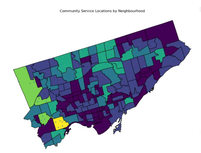
Suppose we want to understand the distribution of Tennis Court Facilities locations across neighbourhoods in Toronto.
We have two Open data sources from the city of Toronto’s Open Data Portal.
- Tennis Courts Facilities — 4326.csv: a table containing service locations, addresses, categories, and coordinates
- Neighbourhoods — 4326.geojson: a boundary file containing Toronto neighbourhood polygons
Our goal is to create a clean geospatial dataset showing the number of service locations in each neighbourhood. A few problematic records are added at the bottom to enable us to validate the data quality.
Pipeline Overview
The workflow follows this structure:

A structured pipeline makes analysis more reliable because each step can be rerun when new data becomes available.
Step 1: Install and Import Libraries
Install the required libraries if they are not already available (assuming you are using a Notebook interface like Jupyter.
#Install  necessary Libraries
%pip install pandas geopandas matplotlib shapely
import pandas as pd
import geopandas as gpd
import matplotlib.pyplot as plt
from pathlib import Path
import json
import shapely
from shapely.geometry import shape
from shapely.geometry.base import BaseGeometry
Step 2: Set Up Project Folders
A clear folder structure makes a project easier to maintain and reproduce.
geospatial_pipeline/
│
├── data/
│   ├── raw/
│   │   ├── Tennis Courts Facilities - 4326.csv
│   │   └── Neighbourhoods - 4326.geojson
│   │
│   └── processed/
│
├── outputs/
│   ├── maps/
│   └── tables/
│
└── scripts/
    └── geospatial_pipeline.py
In Python, define the file paths. Check the current directory and set it to your workspace folder. In my case, I changed my current directory to my current one.
import os
# Check your current directory
print(os.getcwd())
# Change the directory to your workspace folder
os.chdir(r"C:\Users\visha\geospatial_pipeline")
#Define the file paths:
BASE_DIR = Path.cwd()
RAW_DATA = BASE_DIR / "Data" / "Raw"
PROCESSED_DATA = BASE_DIR / "Data" / "Processed"
OUTPUTS = BASE_DIR / "Outputs"
MAPS = OUTPUTS / "Maps"
TABLES = OUTPUTS / "Tables"
for folder in [PROCESSED_DATA, MAPS, TABLES]:
    folder.mkdir(parents=True, exist_ok=True)
Step 3: Load the Raw Data
Load the service-location table and neighbourhood boundary file.
Step 3: Load the Raw Data

#Load the service-location table and neighbourhood boundary file.

services = pd.read_csv(RAW_DATA / "Tennis Courts Facilities - 4326.csv")
neighbourhoods = gpd.read_file(RAW_DATA / "Neighbourhoods - 4326.geojson")

print(services.head())
print(neighbourhoods.head())
#Check the type of the Geometry column
print(type(services["geometry"].iloc[0]))
print(services["geometry"].iloc[0])
Step 4: Convert the geometry column to spatial objects
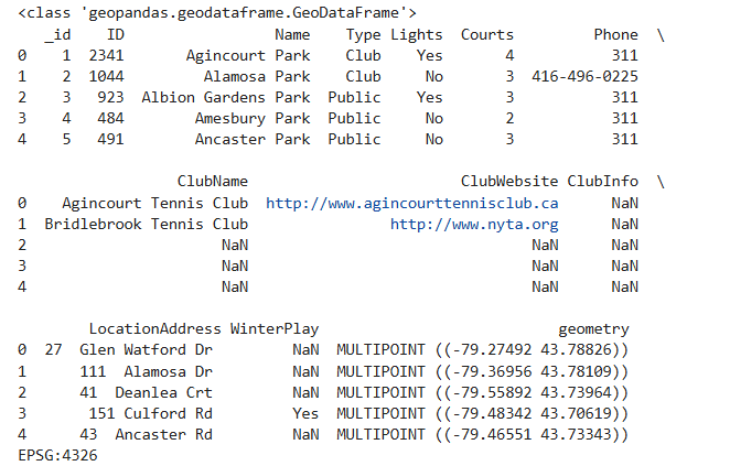
The “services” CSV appears to contain a geometry column in GeoJSON format, so you need to convert that column into Shapely geometry objects before creating a GeoDataFrame.
#This converts  text like JSON into a Shapely MultiPoint geometry.
services["geometry"] = services["geometry"].apply(
    lambda x: shape(json.loads(x))
    if not isinstance(x, BaseGeometry)
    else x
)
#Create the GeoDataFrame
services_gdf = gpd.GeoDataFrame(
    services,
    geometry="geometry",
    crs="EPSG:4326"
)
#verify
print(type(services_gdf))
print(services_gdf.head())
print(services_gdf.crs)
Before analysis, inspect the data structure. This step helps identify missing values, incorrect data types, unexpected fields, and coordinate-system issues.
Step 5: Inspect the data
print(services_gdf.info())
print(services_gdf.isna().sum())

print(neighbourhoods.info())
print(neighbourhoods.crs)
Step 6: Clean and Standardize the Tabular Data
Raw data often contains inconsistent text, duplicate records, and missing coordinates. In the services file, we have 172 records. The ClubInfo column has only one non-null value.
services_gdf.columns = (
    services.columns
    .str.strip()
    .str.lower()
    .str.replace(" ", "_")
)

neighbourhoods.columns = (
    neighbourhoods.columns
    .str.strip()
    .str.lower()
    .str.replace(" ", "_")
)

print(services_gdf.columns)
print(neighbourhoods.columns)
Step 7: Validate Neighbourhood Data Quality
A good data quality check for a GeoDataFrame includes:
- Missing geometries
- Invalid geometries
- Empty geometries
- Correct CRS
- Duplicate neighbourhoods (if applicable)
# Missing geometries
missing_geom = neighbourhoods.geometry.isna().sum()

# Invalid geometries
invalid_geom = (~neighbourhoods.geometry.is_valid).sum()

# Empty geometries
empty_geom = neighbourhoods.geometry.is_empty.sum()

print("Missing geometries:", missing_geom)
print("Invalid geometries:", invalid_geom)
print("Empty geometries:", empty_geom)
neighbourhoods_clean = neighbourhoods[
    neighbourhoods.geometry.notna() &
    neighbourhoods.geometry.is_valid &
    (~neighbourhoods.geometry.is_empty)
].copy()
#Check for duplicate IDS
print("Duplicate AREA_IDs:",
      neighbourhoods_clean["area_id"].duplicated().sum())
#if duplicate exists run this
# neighbourhoods_clean = neighbourhoods_clean.drop_duplicates( subset="area_id")
Step 8: Create a QA summary
qa_summary = pd.DataFrame({
    "metric": [
        "Raw neighbourhoods",
        "Missing geometries",
        "Invalid geometries",
        "Empty geometries",
        "Neighbourhoods retained"
    ],
    "count": [
        len(neighbourhoods),
        missing_geom,
        invalid_geom,
        empty_geom,
        len(neighbourhoods_clean)
    ]
})

print(qa_summary)

qa_summary.to_csv(TABLES / "neighbourhood_quality_summary.csv",
                  index=False)
Step 9: Perform a Spatial Join
A spatial join assigns each service location to the neighbourhood polygon that contains it.
#spatial join
services_with_neighbourhood = gpd.sjoin(
    services_gdf,
    neighbourhoods[["area_name", "geometry"]],
    how="left",
    predicate="within"
)
#Review records that did not match a neighbourhood
unmatched_records = services_with_neighbourhood[
    services_with_neighbourhood["area_name"].isna()
]

print(f"Unmatched records: {len(unmatched_records)}")

#Export unmatched records for review
unmatched_records.to_csv(
    TABLES / "unmatched_service_locations.csv",
    index=False
)
Step 10: Create Neighbourhood-Level Indicators
Next, calculate the number of service locations in each neighbourhood.
Step 11: Export Analysis-Ready Outputs
Export the processed point data, neighbourhood summary, and non-spatial table.
#Export Analysis-Ready Outputs
services_with_neighbourhood.to_file(
    PROCESSED_DATA / "service_locations_with_neighbourhood.geojson",
    driver="GeoJSON"
)

neighbourhood_summary.to_file(
    PROCESSED_DATA / "neighbourhood_service_summary.geojson",
    driver="GeoJSON"
)

neighbourhood_summary.drop(columns="geometry").to_csv(
    TABLES / "neighbourhood_service_summary.csv",
    index=False
)
These outputs can now be used in ArcGIS, Power BI, Tableau, QGIS, Web maps, etc.,
Step 12: Create a Quality-Assurance Map
Maps are not only communication tools; they are also useful for checking whether the spatial join and geographic patterns make sense.
neighbourhood_summary.plot(
    column="service_count",
    legend=True,
    ax=ax,
    edgecolor="black"
)

services_gdf.plot(
    ax=ax,
    markersize=8,
    alpha=0.6
)

ax.set_title("Community Service Locations by Neighbourhood")
ax.set_axis_off()

plt.tight_layout()
plt.savefig(MAPS / "service_locations_by_neighbourhood.png", dpi=300)
plt.show()
When reviewing the map, check for: Points located outside the city boundary, Unexpected clusters, Missing neighbourhood assignments, Areas with zero services, Duplicate point locations, Patterns that may require further investigation.
Stpe 13: Make the Pipeline Reusable
The strongest data pipelines are repeatable. Instead of manually repeating each step, place the workflow in a Python script and rerun it when new data arrives.
# Make the Pipeline Reusable

def load_data():
    pass

def clean_data(data):
    pass

def validate_data(data):
    pass

def create_geodataframe(data):
    pass

def spatial_join(points, boundaries):
    pass

def create_summary(joined_data, boundaries):
    pass

def export_outputs(points, summary):
    pass
This approach makes the workflow easier to test, troubleshoot, document, and maintain. This tutorial demonstrated how Python can support an end-to-end geospatial data workflow:
- Ingest raw tabular and spatial data
- Clean and standardize fields
- Validate records before analysis
- Convert coordinates into geographic features
- Perform spatial joins
- Create neighbourhood-level indicators
- Export analysis-ready datasets
- Use maps for quality assurance and decision-making
A well-designed geospatial pipeline improves data reliability, supports reproducible analysis, and makes it easier for organizations to turn location data into actionable insights.
I hope you’ve made it to the end of this article and are interested in replicating this work. I’ve uploaded the notebook to my GitHub repository, where you can download it and recreate the analysis yourself.